Playing Atari with Deep Reinforcement Learning

Context (title): Playing Atari with Deep Reinforcement Learning

This paper by Volodymyr Mnih, presented at NIPS 2013, is essentially the pioneering work of DQN. Another significant paper is the Nature 2015 article “Human-level control through deep reinforcement learning.” Both papers are considered milestones in the field of reinforcement learning. This article will summarize some of the groundbreaking ideas presented in the NIPS 2013 paper.

Abstract

This is the first paper to use a deep learning model to directly learn control strategies from high-dimensional sensor inputs through reinforcement learning. The model is built on a CNN and learns using a variant of Q-learning. The input is raw pixels, representing the current state, and the output is the Q-value, essentially using a neural network to approximate the Q(s,a) function. The paper conducted experiments on Atari 2600 games, achieving excellent results without special adjustments to the structure and algorithm, outperforming previous algorithms and human performance.

1. Introduction

Learning control strategies directly from high-dimensional sensor data (such as speech and images) has been a long-standing challenge for RL. Most successful RL applications require manual feature tuning, making their effectiveness heavily dependent on the quality of feature selection. However, deep learning makes it possible to extract features from high-dimensional data, suggesting that combining the two could yield excellent results.

However, using deep learning for RL presents many challenges. Current deep learning heavily relies on manually labeled data, while RL does not have this direct one-to-one relationship. Instead, it requires many iterations to obtain a scalar reward, which is often sparse, noisy, and significantly delayed. In RL, it usually takes thousands of steps to receive a reward, making it appear very sluggish compared to the conventional one-to-one data-label scenario. Additionally, deep learning often requires training data to be independent, whereas RL data is a highly interdependent sequence of states. As RL learns new actions, the data distribution changes, which can lead to pathological effects for deep learning algorithms that require a fixed data distribution. The main issues are data correlation and data distribution.

This paper proposes a CNN-based network structure that introduces an experience replay mechanism to mitigate data correlation and distribution issues. Experience replay smooths the data distribution by randomly sampling transitions. During training, the model receives the same data as humans, including video input, rewards, termination signals, and possible action sets.

2. Background

The Atari simulator used for training here requires attention to the fact that the reward, or game score, depends on the previous action sequence and observations, with feedback possibly received only after thousands of steps. A single screen observation cannot fully understand the current state, so a sequence is needed to represent the current state, i.e., $s_{t}=x_{1},a_{1},x_{2},...,a_{t-1},x_{t}$. A sequence of screen observations and actions represents the current state, and these sequences are used to learn game strategies. All sequences in the simulator are assumed to terminate within a finite number of time steps, allowing standard reinforcement learning methods to be applied to these sequences.

Additionally, it is assumed that the reward decreases over time steps, using a discount factor to process the reward, with cumulative reward $R_{t}=\sum^{T}_{t'=t}\gamma^{t'-t}r_{t'}$, where $T$ is the termination time step of the game. Define $Q^{*}(s,a)$ as the Q-value function under the optimal strategy, i.e., $Q^{*}(s,a)=max_{\pi}E[R_{t}|s_{t}=s,a_{t}=a,\pi]$. The optimal Q-function follows the Bellman equation: if $Q(s',a')$ is known for the next sequence $s'$ and all possible actions $a'$, then $Q^{*}(s,a)$ maximizes the expectation $r+\gamma Q^{*}(s',a')$, i.e.,

$$Q^{*}(s,a)=E_{s'\sim \varepsilon}[r+\gamma max_{a'}Q^{*}(s',a')|s,a]$$

Many RL algorithms aim to estimate the Q-value function. If the Bellman equation is iteratively used, $Q_{i+1}(s,a)=E[r+\gamma max_{a'}Q_{i}(s',a')|s,a]$, it can eventually converge to $Q^*$ as $i\to\infin$. However, in practice, this is impractical because the Q-function is estimated separately for each sequence, lacking generalization. Instead, a function is used to approximate the optimal Q-function, i.e., $Q(s,a;\theta)=Q^*(s,a)$. Here, a neural network is used for estimation, with the loss function:

$$L_{i}(\theta_{i})=E_{s,a\sim p(\cdot)}[(y_{i}-Q(s,a;\theta_{i}))^2]$$

where $y_{i}=E_{s'\sim \varepsilon}[r+\gamma max_{a'}Q(s',a';\theta_{i-1})|s,a]$. In code implementation, $Q(s,a;\theta_{i})$ and $Q(s,a;\theta_{i-1})$ are usually defined using two different networks. In PyTorch tutorials, policy_net and target_net are used. Additionally, a certain probability is used to balance “exploration” and “exploitation” during action selection, i.e., the $\epsilon$-greedy algorithm. At the start of training, actions with high returns are utilized, while more exploration is conducted later, with $\epsilon$ decaying from large to small.

3. Related Work

This section will be supplemented once the purchased book arrives.

4. Deep Reinforcement Learning

This chapter mainly introduces the core algorithm. First, it is important to recognize that using deep learning for feature extraction is superior to manual feature processing. The pseudocode for the DQN algorithm framework is as follows: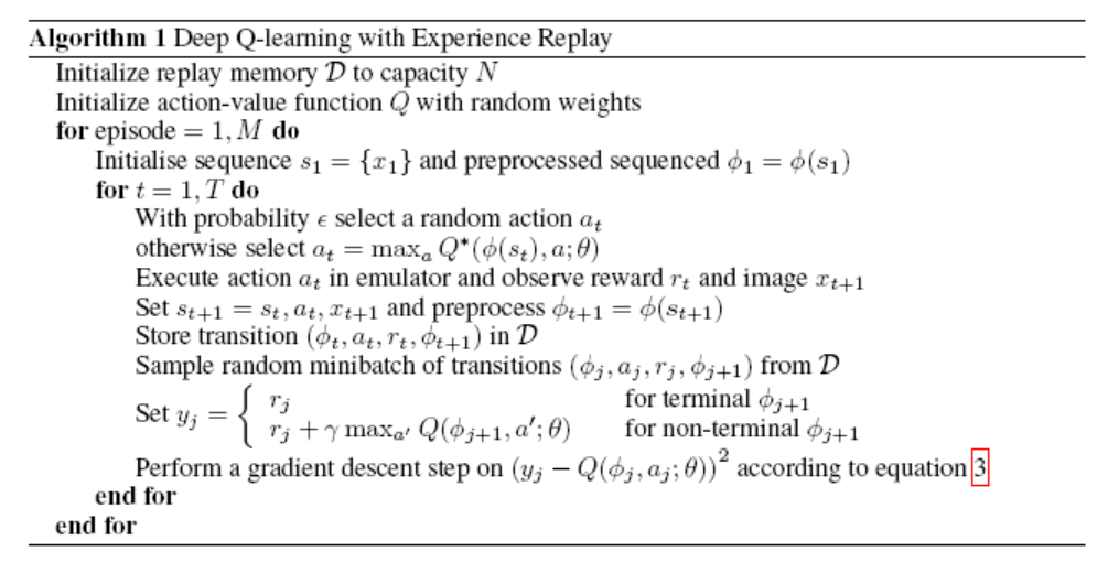

The benefits of replay memory are reintroduced here: 1. Each state transition can potentially be used for network weight updates. 2. Due to the strong correlation between samples, learning directly from consecutive samples is inefficient. Breaking this correlation and performing random sampling can reduce bias during updates. 3. In learning on-policy, the current parameters generate the next batch of samples for parameter updates. For example, if the action with the highest reward under current parameters is moving left, subsequent samples will always be left. If the best action later becomes moving right, the training distribution will also change, easily leading to a vicious cycle and local optima. Replay allows behavior distribution to average across multiple previous states, smoothing the learning process and preventing divergence. Therefore, learning off-policy is necessary, distinguished by whether the policy generating actions and the policy updating network parameters are the same. In Q-learning, the policy used during updates employs the max operation, while the policy generating actions may not always use the action with the highest reward. Q-learning is a classic off-policy learning algorithm.

For the neural network here, the state is used as input, and the n output nodes correspond to the rewards caused by n possible actions, allowing the reward for each action to be calculated in one computation.

The subsequent experimental chapter is not elaborated on due to the passage of time.