Quantitative Analysis of Accelerating PyTorch Training

Training neural networks is often the most time-consuming part of the entire process, especially when training a randomly initialized neural network to convergence on a large dataset. Generally speaking, using better hardware platforms can speed up the training process, such as using more and better GPUs, larger and faster SSDs, and replacing Ethernet with InfiniBand for distributed training. Besides hardware, software and algorithms are equally crucial; a good software platform should make full use of the existing hardware resources. This article starts with a baseline and gradually optimizes the training speed through various methods. Our chosen baseline is training ResNet18 on the ImageNet dataset for a total of 90 epochs, with the initial computing platform as shown in Table 1:

Alt text — Table 1: Baseline Configuration

1. Analyzing Time Bottlenecks in the Training Process

We use the NVIDIA Tools Extension Library (NVTX) to measure the time costs of various parts during the training process. The usage is simple: just insert a few lines of code into the training script and start training with nsys profile python3 main.py. This will generate a .qdrp file. We recorded the time spent on data loading, forward propagation, backward propagation, and gradient descent for one batch. To save time, we collected statistics for 300 batches.

import torch.cuda.nvtx as nvtx
nvtx.range_push("Batch 0")
nvtx.range_push("Load Data")
for i, (input_data, target) in enumerate(train_loader):
    input_data = input_data.cuda(non_blocking=True)
    target = target.cuda(non_blocking=True)
    nvtx.range_pop(); nvtx.range_push("Forward")
    output = model(input_data)
    nvtx.range_pop(); nvtx.range_push("Calculate Loss/Sync")
    loss = criterion(output, target)
    prec1, prec5 = accuracy(output, target, topk=(1, 5))
    optimizer.zero_grad()
    nvtx.range_pop(); nvtx.range_push("Backward")
    loss.backward()
    nvtx.range_pop(); nvtx.range_push("SGD")
    optimizer.step()
    nvtx.range_pop(); nvtx.range_pop()
    nvtx.range_push("Batch " + str(i+1)); nvtx.range_push("Load Data")
nvtx.range_pop()
nvtx.range_pop()

When training with the baseline code, we visualized the generated .qdrp file using Nvidia Nsight Systems. As shown in Figure 1, the time taken for 300 batches is 336.524s. Notably, the actual running time of the CUDA kernels only accounts for about a quarter of the total time, while three-quarters of the time is spent on data loading. During this process, the CUDA kernel and CPU utilization are almost zero, which becomes a performance bottleneck in our baseline training process.

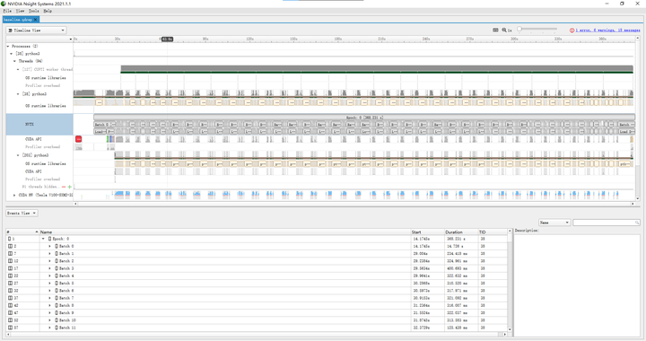
Further examination of the training time for each batch (e.g., batch 122) shows that transferring data from Host memory to Device memory takes 13.6ms (data size is 224*224*3*256*4=154,140,672 bytes, bandwidth 11.3GB/s); forward propagation with CUDA kernel takes 15.4ms, actual CUDA kernel running time is 67.3ms; backward propagation with CUDA kernel takes 19.9ms, actual CUDA kernel running time is 164.7ms; SGD with CUDA kernel takes 8.0ms, actual CUDA kernel running time is 1.8ms.

2. Accelerating Data Loading

From the results of the previous section, it is evident that three-quarters of the training time is spent on data loading, during which CPU/GPU utilization is almost zero, leading to a waste of hardware resources. Therefore, we first optimize the I/O part. The slow data loading in the baseline training code is mainly because PyTorch reads raw images in formats like .jpeg during training, which requires decoding and non-sequential reading, resulting in many cache misses and long I/O times. In contrast, frameworks like TensorFlow have their own .tfrecord format, similar to hdf5, lmdb, etc., which store the entire dataset in a large binary file, allowing for sequential reading and much higher efficiency.

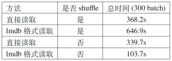
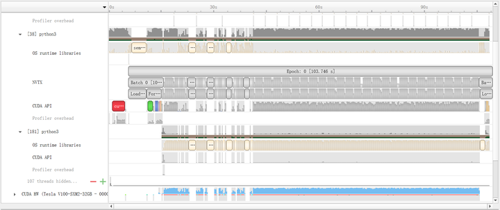
When optimizing I/O, the choice of solution should depend on the hardware environment. If the computing platform’s memory cannot accommodate the entire dataset, lmdb can be used (hdf5 requires loading the entire file into memory). We conducted two sets of experiments for comparison: random reading (shuffle training data) and sequential reading (no shuffle). The results are shown in Table 2. If the dataset is not shuffled, reading with lmdb is very fast. The profile results in Figure 2 show that after training about 50 batches, the CUDA kernel is almost always busy, thanks to the reduced cache miss rate from sequential reading. However, with shuffling, it becomes slower.

If the memory is large enough, the entire dataset can be directly placed in memory. This can be achieved by mounting a tmpfs file system and placing the entire dataset in that folder. If mounting permissions are not available, the dataset can be placed in the /dev/shm directory, which is also a tmpfs file system. Typically, 160G is enough to accommodate the entire ImageNet dataset.

# With mounting permissions
mkdir -p /userhome/memory_data/imagenet
mount -t tmpfs -o size=160G tmpfs /userhome/memory_data/imagenet
root_dir="/userhome/memory_data/imagenet"
# Without mounting permissions
mkdir -p /dev/shm/imagenet
root_dir="/dev/shm/imagenet"
mkdir -p "${root_dir}/train"
mkdir -p "${root_dir}/val"
tar -xvf /userhome/data/ILSVRC2012_img_train.tar -C "${root_dir}/train"
tar -xvf /userhome/data/ILSVRC2012_img_val.tar -C "${root_dir}/val"

After placing the dataset in the tmpfs file system, we retrained using the baseline code. As shown in Figure 3, the CUDA kernel is almost always fully loaded, and the overall training time is reduced from the baseline 336.524s to 87.989s (only 26% of the baseline), demonstrating a significant speedup.

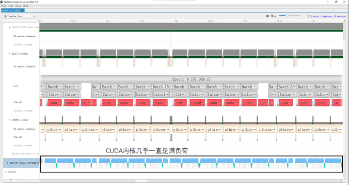
Similarly, we further analyzed the training time for each batch. Transferring data from Host memory to Device memory takes 15.4ms (1.8ms ↑); forward propagation with CUDA kernel takes 7.9ms (7.5ms ↓), actual CUDA kernel running time is 67.5ms (0.2ms ↑); backward propagation with CUDA kernel takes 16.6ms (3.3ms ↑), actual CUDA kernel running time is 164.3ms (0.4ms ↑); SGD with CUDA kernel takes 5.5ms (2.5ms ↑), actual CUDA kernel running time is 1.9ms (0.1ms ↑). It can be seen that the computation time is almost the same as the baseline.

3. Mixed Precision Training

From the previous section, it is clear that after optimizing data loading, the CUDA kernel can be fully loaded. Therefore, to further speed up training, we must focus on the computation speed itself (mainly forward and backward), but since PyTorch uses CUDNN kernels for computation, we cannot optimize the kernels themselves. Instead, we can speed up by converting some FP32 computations to FP16, i.e., mixed precision training.

A relatively simple way to implement mixed precision training is to use Apex (A PyTorch Extension), which requires adding only a few lines of code to the original script and allows choosing different FP16 training schemes.

from apex import amp, optimizers
# Allow Amp to perform casts as required by the opt_level
model, optimizer = amp.initialize(model, optimizer, opt_level="O1")
...
# loss.backward() becomes:
with amp.scale_loss(loss, optimizer) as scaled_loss:
    scaled_loss.backward()
...

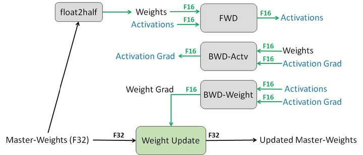
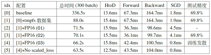
The opt_level has several options: O0 uses FP32 for all training, O1 uses FP16 for some operations, O2 uses FP16 for most operations, and O3 uses FP16 for all operations. When using O1 and O2, FP16 operators (convolution, fully connected, etc.) use FP16 for forward and backward propagation but maintain an FP32 weight for gradient descent updates (Figure 4). FP32 operators (BN, etc.) use FP32 for forward and backward propagation. Note that both types of operators use FP32 for gradient descent. Training with FP16 carries some risk of divergence, so the choice of scheme should balance speedup and preventing divergence based on the actual situation. We conducted experiments on FP16 training based on the fastest scheme from the previous section, and the results are shown in Table 3. It can be seen that using FP16 for training significantly improves the speed of forward and backward compared to FP32, and the overall training time also decreases noticeably.

Up to this section, we have been using a single GPU for training. The training speed of the neural network has been gradually increased by various methods, starting from the baseline 336.524s (Figure 1), accelerated to 87.989s after I/O optimization (Figure 3), and further accelerated to 70.1s using mixed precision training without reducing accuracy.

4. Single Machine Multi-GPU Parallel Training

In this section, we will further accelerate training by using single machine multi-GPU parallel training, based on optimized data loading and mixed precision training. We will focus on data parallelism for now, without considering model parallelism or even operator parallelism.

There are two common ways to implement single machine multi-GPU training in PyTorch: using nn.DataParallel or nn.parallel.DistributedDataParallel. The former uses a single process, while the latter uses multiple processes for parallel training, also suitable for multi-machine multi-GPU scenarios. Besides nn.parallel.DistributedDataParallel, there are third-party libraries for multi-process parallel training in PyTorch, such as APEX and Horovod.

Using nn.DataParallel is the simplest method, requiring only one line of code:

model = torch.nn.DataParallel(model)

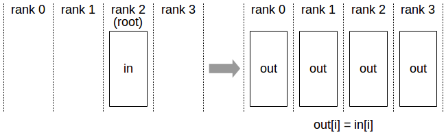
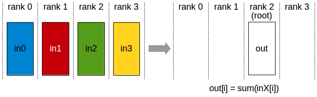
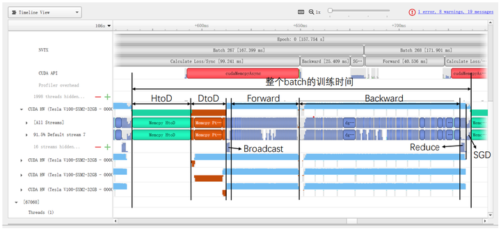
When using nn.DataParallel for parallel training, the entire batch of data is first loaded onto a primary GPU, and then each portion of data (BS/GPU_NUM) is copied from the primary GPU to other GPUs via PtoP. Then, the model parameters are broadcast from the primary GPU to other GPUs using the NVIDIA Collective Communications Library (NCCL) (Figure 5). Each GPU then performs forward and backward propagation independently, and finally, the gradients from other GPUs are reduced to the primary GPU, which performs gradient descent to obtain the optimized neural network.

We first conducted experiments based on configuration [1] and used the same batch size (e.g., when the total batch size is 256, each card uses 128 with two cards, and 64 with four cards). The results are shown in Table 4 (the experiment iterated 500 batches, with the total time for the middle 300 batches recorded in Table 4; DtoD time includes two parts: the time for the primary GPU to PtoP each portion of data to other GPUs, and the total time for broadcasting model parameters from the primary GPU and reducing gradients to the primary GPU). The profile results for BS=512 are shown in Figure 7.

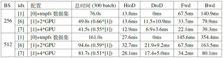
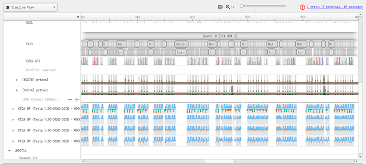
From Table 4 and Figure 7, several observations can be made:

Using multiple GPUs can effectively reduce the time for forward and backward propagation.
When the number of GPUs increases to a certain extent, there will be a waiting period for data loading after GPU computation is complete.
As the number of GPUs increases, the time spent on communication between GPUs becomes a larger proportion, and the speed improvement from increasing the number of GPUs becomes limited.

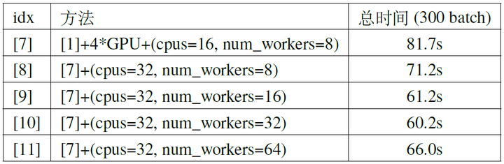
For the second point, the data loading time consists of two parts: I/O time, which we have addressed by placing the dataset in memory, and data preprocessing time, which can be addressed by increasing the number of CPU threads and data loading threads. When training in a Docker container, the former can be achieved by modifying the --cpus parameter in docker run, and the latter by appropriately increasing the num_workers parameter when creating a torch.utils.data.DataLoader object. We further improved configuration [7], and the experimental results for BS=512 are shown in Table 5. It can be seen that if there is still idle time waiting for data during training, appropriately increasing the number of CPU threads and data loading threads can effectively reduce the total time (mainly by reducing the idle time waiting for data), but excessively increasing the number of threads can lead to some waste, as the idle time waiting for data becomes very small. Additionally, excessively increasing the number of threads can become slower due to the overhead of the threads themselves (e.g., [10] and [11] in the table).

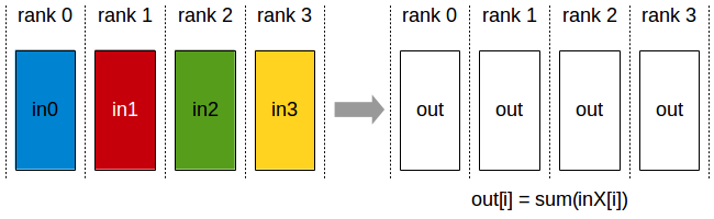
For the third point, note that nn.DataParallel first transfers all data from memory to a primary GPU, and then PtoP transfers each portion of data from the primary GPU to other GPUs. This process is not as efficient as directly transferring each portion of data from memory to the corresponding GPU, which can save the time spent transferring each portion of data from the primary GPU to other GPUs via PtoP (the first part of DtoD time in Table 5, accounting for nearly 20% in configuration [7]). Additionally, nn.DataParallel broadcasts model parameters from the primary GPU to other GPUs at the beginning of each iteration and reduces gradients to the primary GPU at the end. Using All-Reduce to distribute the reduced gradients to each GPU (Figure 8) allows each GPU to perform gradient descent independently, saving the initial time cost of broadcasting model parameters in nn.DataParallel (approximately 2%).

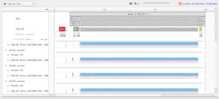
The multi-process based nn.parallel.DistributedDataParallel implements this method. For usage details, refer to the official example. We conducted experiments based on configuration [10], and the results are shown in Table 6. The DtoD time for DistributedDataParallel was not recorded due to significant fluctuations in synchronization time between different GPUs. It can be seen that using DistributedDataParallel can reduce the time by about one-third. The profile results (Figure 9) show that the CUDA kernel utilization in configuration [12] is much higher than in configuration [7], partly due to the use of more CPU and data loading threads and partly due to the multi-process parallel training implementation, which can bypass Python’s GIL (Global Interpreter Lock) and further improve efficiency.

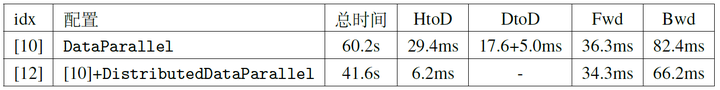
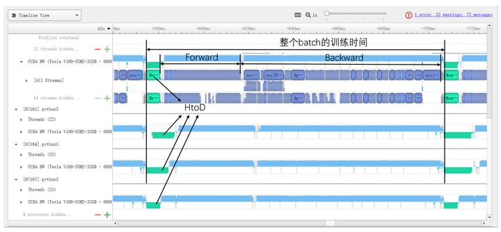
Specifically, Figures 10 and 11 show the specific time costs for training a batch using DataParallel and DistributedDataParallel, respectively. When using DistributedDataParallel, the data size for HtoD in Figure 9 is reduced from the total BS to BS/GPU_NUM, theoretically reducing the time to 1/GPU_NUM of DataParallel (with slight fluctuations in transfer speed between different GPUs). Additionally, the DtoD time can be completely saved, and the time for Broadcast and Reduce is replaced by All-Reduce (with significant fluctuations due to synchronization across all GPUs). The computation time (Forward/Backward/SGD) for these two methods shows no significant difference.

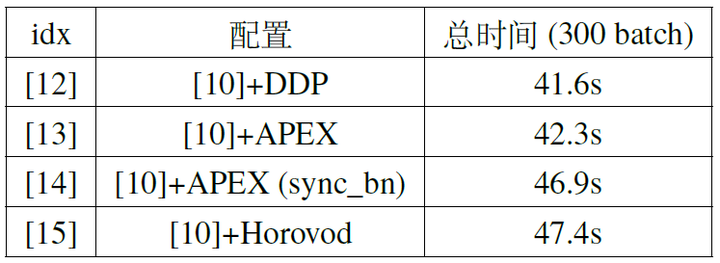
In addition to DistributedDataParallel, we previously mentioned that APEX and Horovod are third-party libraries that implement the same multi-process parallelism. We also conducted comparative experiments using these two third-party libraries, and the results are shown in Table 7. It can be seen that the speed differences between the three implementations are not significant. Notably, APEX can perform synchronized operations on BN, meaning that when calculating the mean/standard deviation for the BN layer, data from all GPUs is synchronized, resulting in mean/standard deviation statistics from the entire batch rather than from a single GPU’s portion. This approach can make training more stable. However, this method requires synchronization (sync) across all GPUs when calculating the mean/variance, resulting in some additional time overhead. However, from the profile results, the main reason for GPU computation desynchronization is the initial HtoD time difference, and after synchronization at the first BN layer, the subsequent BN layers require very short synchronization times (assuming all GPUs have similar computational power).

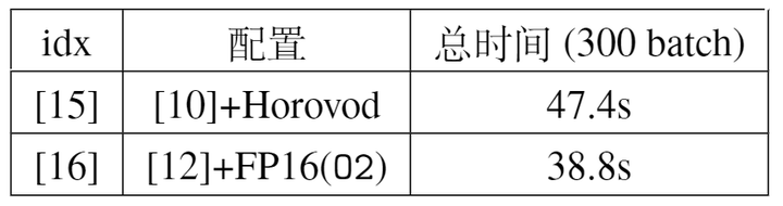
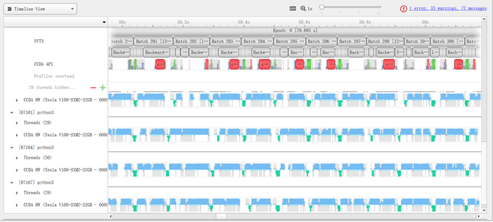
Finally, we combine the mixed precision training from the previous section with the multi-GPU training method from this section. By combining these two orthogonal acceleration methods, we can push the training speed to the limit. Specifically, Table 8 shows that using DistributedDataParallel achieves the highest parallel efficiency, so we combine it with FP16(O2). Experimental results show that this method can further accelerate to 38.8s, with the profile results shown in Figure 12.

5. Multi-Machine Multi-GPU Parallel Training

The previous experiments were conducted on a single machine, but in practice, distributed training across multiple machines is needed for further acceleration. For example, in a dual-machine four-GPU setup, training can be conducted with the following code:

# Assuming running on 2 machines, each with 4 available GPUs
#    Machine 1:
python -m torch.distributed.launch --nnodes=2 --node_rank=0 --nproc_per_node 4 \
  --master_adderss $my_address --master_port $my_port main.py
#    Machine 2:
python -m torch.distributed.launch --nnodes=2 --node_rank=1 --nproc_per_node 4 \
  --master_adderss $my_address --master_port $my_port main.py

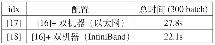
We tested the training speed under different hardware configurations, mainly differing in whether InfiniBand was used. The experimental results are shown in Table 9. Since data synchronization between machines is required during training, part of the training time comes from inter-machine communication. Using InfiniBand can achieve lower latency than Ethernet (though Ethernet is more versatile, InfiniBand is relatively more suitable for parallel computing scenarios).

6. Summary

In this article, we optimized training step by step by adjusting configurations to make full use of GPU computing power. Initially, using the baseline code, a single GPU, and BS=512, training 300 batches took 161.0s (Configuration [0]). Then, using DataParallel for training on 4 GPUs accelerated it to 81.7s (Configuration [7]). Further increasing CPU threads and data loading threads accelerated it to 60.2s (Configuration [10]). Additionally, replacing DataParallel with DistributedDataParallel reduced GPU communication time, accelerating it to 41.6s (Configuration [12]). Combining this with mixed precision training further accelerated it to 38.8s (Configuration [16]). Finally, using two such nodes for parallel training with InfiniBand communication accelerated it to 22.1s (Configuration [18]).